Examples
A step-by-step basic example
This example shows the basic usage of getfem, on the über-canonical problem above
all others: solving the Laplacian, \(-\Delta u = f\) on a square,
with the Dirichlet condition \(u = g(x)\) on the domain boundary. You can find
the py-file of this example under the name demo_step_by_step.py in the
directory interface/tests/python/ of the GetFEM distribution.
The first step is to create a Mesh object. It is possible to create simple structured meshes or unstructured meshes for simple geometries (see getfem.Mesh('generate', mesher_object mo, scalar h)) or to rely on an external mesher (see getfem.Mesh('import',
string FORMAT, string FILENAME)), or use very simple meshes. For this example,
we just consider a regular meshindex{cartesian mesh} whose nodes are
\(\{x_{i=0\ldots10,j=0..10}=(i/10,j/10)\}\)
1# import basic modules
2import numpy as np
3import getfem as gf
4
5# creation of a simple cartesian mesh
6m = gf.Mesh('cartesian', np.arange(0,1.1,0.1), np.arange(0,1.1,0.1))
The next step is to create a MeshFem object. This one links a mesh with a set of FEM
1# create a MeshFem of for a field of dimension 1 (i.e. a scalar field)
2mf = gf.MeshFem(m, 1)
3# assign the Q2 fem to all convexes of the MeshFem
4mf.set_fem(gf.Fem('FEM_QK(2,2)'))
The first instruction builds a new MeshFem object, the second argument specifies that this object will be used to interpolate scalar fields (since the unknown \(u\) is a scalar field). The second instruction assigns the \(Q^2\) FEM to every convex (each basis function is a polynomial of degree 4, remember that \(P^k\rm I\hspace{-0.15em}Rightarrow\) polynomials of degree \(k\), while \(Q^k\rm I\hspace{-0.15em}Rightarrow\) polynomials of degree \(2k\)). As \(Q^2\) is a polynomial FEM, you can view the expression of its basis functions on the reference convex:
1# view the expression of its basis functions on the reference convex
2print gf.Fem('FEM_QK(2,2)').poly_str()
Now, in order to perform numerical integrations on mf, we need to build a
MeshIm object
1# an exact integration will be used
2mim = gf.MeshIm(m, gf.Integ('IM_EXACT_PARALLELEPIPED(2)'))
The integration method will be used to compute the various integrals on each
element: here we choose to perform exact computations (no quadrature
formula), which is possible since the geometric transformation of these convexes
from the reference convex is linear (this is true for all simplices, and this is
also true for the parallelepipeds of our regular mesh, but it is not true for
general quadrangles), and the chosen FEM is polynomial. Hence it is possible to
analytically integrate every basis function/product of basis
functions/gradients/etc. There are many alternative FEM methods and integration
methods (see User Documentation).
Note however that in the general case, approximate integration methods are a better choice than exact integration methods.
Now we have to find the <boundary> of the domain, in order to
set a Dirichlet condition. A mesh object has the ability to store some sets of
convexes and convex faces. These sets (called <regions>) are accessed via an
integer #id
1# detect the border of the mesh
2border = m.outer_faces()
3# mark it as boundary #42
4m.set_region(42, border)
Here we find the faces of the convexes which are on the boundary of the mesh (i.e. the faces which are not shared by two convexes).
The array border has two rows, on the first row is a convex number, on the
second row is a face number (which is local to the convex, there is no global
numbering of faces). Then this set of faces is assigned to the region number 42.
At this point, we just have to describe the model and run the solver to get the
solution! The “model” is created with the Model constructor. A model
is basically an object which build a global linear system (tangent matrix for
non-linear problems) and its associated right hand side. Typical modifications are
insertion of the stiffness matrix for the problem considered (linear elasticity,
laplacian, etc), handling of a set of constraints, Dirichlet condition, addition of
a source term to the right hand side etc. The global tangent matrix and its right
hand side are stored in the “model” structure.
Let us build a problem with an easy solution: \(u = x(x-1)-y(y-1)\), then we have \(-\Delta u = 0\) (the FEM won’t be able to catch the exact solution since we use a \(Q^2\) method).
We start with an empty real model
1# empty real model
2md = gf.Model('real')
(a model is either 'real' or 'complex'). And we declare that u is an
unknown of the system on the finite element method mf by
1# declare that "u" is an unknown of the system
2# on the finite element method `mf`
3md.add_fem_variable('u', mf)
Now, we add a generic elliptic brick, which handles \(-\nabla\cdot(A:\nabla
u) = \ldots\) problems, where \(A\) can be a scalar field, a matrix field, or
an order 4 tensor field. By default, \(A=1\). We add it on our main variable
u with
1# add generic elliptic brick on "u"
2md.add_Laplacian_brick(mim, 'u');
Next we add a Dirichlet condition on the domain boundary
1# add Dirichlet condition
2g = mf.eval('x*(x-1) - y*(y-1)')
3md.add_initialized_fem_data('DirichletData', mf, g)
4md.add_Dirichlet_condition_with_multipliers(mim, 'u', mf, 42, 'DirichletData')
The two first lines defines a data of the model which represents the value of the
Dirichlet condition. The third one add a Dirichlet condition to the variable u
on the boundary number 42. The dirichlet condition is imposed with lagrange
multipliers. Another possibility is to use a penalization. A MeshFem argument is
also required, as the Dirichlet condition \(u=g\) is imposed in a weak form
\(\int_\Gamma u(x)v(x) = \int_\Gamma g(x)v(x)\ \forall v\) where \(v\) is
taken in the space of multipliers given by here by mf.
Remark:
the polynomial expression was interpolated on mf. It is possible only if
mf is of Lagrange type. In this first example we use the same MeshFem for
the unknown and for the data such as g, but in the general case, mf
won’t be Lagrangian and another (Lagrangian) MeshFem will be used for the
description of Dirichlet conditions, source terms etc.
A source term can be added with (uncommented) the following lines
1# add source term
2#f = mf.eval('0')
3#md.add_initialized_fem_data('VolumicData', mf, f)
4#md.add_source_term_brick(mim, 'u', 'VolumicData')
It only remains now to launch the solver. The linear system is assembled and solve with the instruction
1# solve the linear system
2md.solve()
The model now contains the solution (as well as other things, such as the linear system which was solved). It is extracted
1# extracted solution
2u = md.variable('u')
Then export solution
1# export computed solution
2mf.export_to_pos('u.pos',u,'Computed solution')
and view with gmsh u.pos, see figure Computed solution.
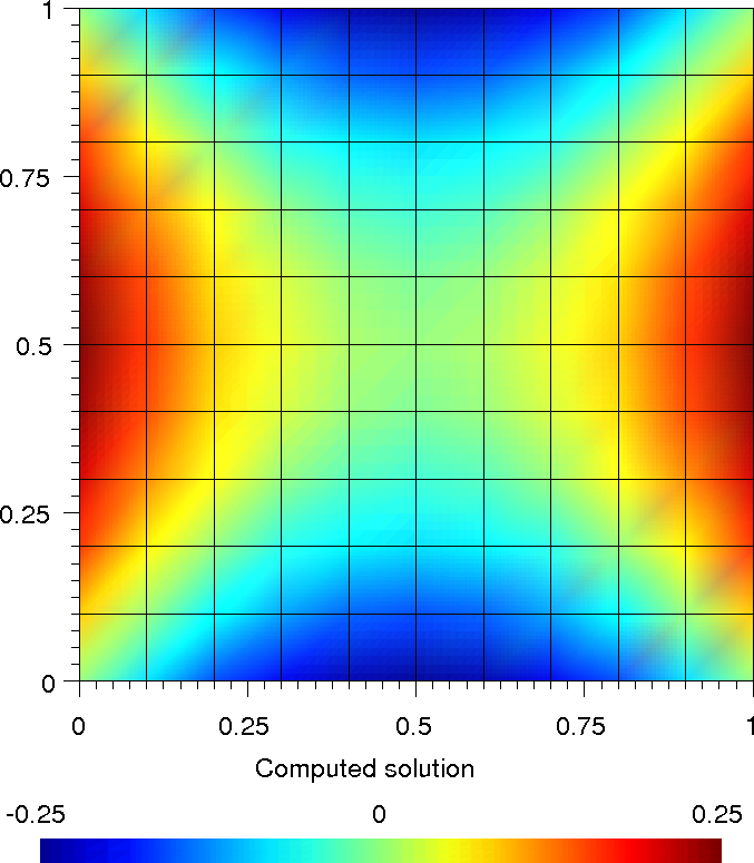
Computed solution
Another Laplacian with exact solution (source term)
This example shows the basic usage of getfem, on the canonical problem: solving
the Laplacian, \(-\Delta u = f\) on a square, with the Dirichlet condition
\(u = g(x)\) on the domain boundary \(\Gamma_D\) and the Neumann condition
\(\frac{\partial u}{\partial\eta} = h(x)\) on the domain boundary
\(\Gamma_N\). You can find the py-file of this example under the name
demo_laplacian.py in the directory interface/tests/python/ of the GetFEM
distribution.
We create Mesh, MeshFem, MeshIm object and find the boundary of the domain in the same way as the previous example
 1import numpy as np
 2
 3# import basic modules
 4import getfem as gf
 5
 6# boundary names
 7top   = 101 # Dirichlet boundary
 8down  = 102 # Neumann boundary
 9left  = 103 # Dirichlet boundary
10right = 104 # Neumann boundary
11
12# parameters
13NX = 40                             # Mesh parameter
14Dirichlet_with_multipliers = True;  # Dirichlet condition with multipliers or penalization
15dirichlet_coefficient = 1e10;       # Penalization coefficient
16
17# mesh creation
18m = gf.Mesh('regular_simplices', np.arange(0,1+1./NX,1./NX), np.arange(0,1+1./NX,1./NX))
19
20# create a MeshFem for u and rhs fields of dimension 1 (i.e. a scalar field)
21mfu   = gf.MeshFem(m, 1)
22mfrhs = gf.MeshFem(m, 1)
23# assign the P2 fem to all convexes of the both MeshFem
24mfu.set_fem(gf.Fem('FEM_PK(2,2)'))
25mfrhs.set_fem(gf.Fem('FEM_PK(2,2)'))
26
27# an exact integration will be used
28mim = gf.MeshIm(m, gf.Integ('IM_TRIANGLE(4)'))
29
30# boundary selection
31flst   = m.outer_faces()
32fnor   = m.normal_of_faces(flst)
33ttop   = abs(fnor[1,:]-1) < 1e-14
34tdown  = abs(fnor[1,:]+1) < 1e-14
35tleft  = abs(fnor[0,:]+1) < 1e-14
36tright = abs(fnor[0,:]-1) < 1e-14
37ftop   = np.compress(ttop, flst, axis=1)
38fdown  = np.compress(tdown, flst, axis=1)
39fleft  = np.compress(tleft, flst, axis=1)
40fright = np.compress(tright, flst, axis=1)
41
42# mark it as boundary
43m.set_region(top, ftop)
44m.set_region(down, fdown)
45m.set_region(left, fleft)
then, we interpolate the exact solution and source terms
1
2# interpolate the exact solution (assuming mfu is a Lagrange fem)
3g = mfu.eval('y*(y-1)*x*(x-1)+x*x*x*x*x')
4
5# interpolate the source terms (assuming mfrhs is a Lagrange fem)
6f = mfrhs.eval('-(2*(x*x+y*y)-2*x-2*y+20*x*x*x)')
and we bricked the problem as in the previous example
 1
 2# model
 3md = gf.Model('real')
 4
 5# add variable and data to model
 6md.add_fem_variable('u', mfu)              # main unknown
 7md.add_initialized_fem_data('f', mfrhs, f) # volumic source term
 8md.add_initialized_fem_data('g', mfrhs, g) # Dirichlet condition
 9md.add_initialized_fem_data('h', mfrhs, h) # Neumann condition
10
11# bricked the problem
12md.add_Laplacian_brick(mim, 'u')                             # laplacian term on u
13md.add_source_term_brick(mim, 'u', 'f')                      # volumic source term
14md.add_normal_source_term_brick(mim, 'u', 'h', down)         # Neumann condition
15md.add_normal_source_term_brick(mim, 'u', 'h', left)         # Neumann condition
16
17# Dirichlet condition on the top
18if (Dirichlet_with_multipliers):
19  md.add_Dirichlet_condition_with_multipliers(mim, 'u', mfu, top, 'g')
20else:
21  md.add_Dirichlet_condition_with_penalization(mim, 'u', dirichlet_coefficient, top, 'g')
22
23# Dirichlet condition on the right
24if (Dirichlet_with_multipliers):
25  md.add_Dirichlet_condition_with_multipliers(mim, 'u', mfu, right, 'g')
26else:
the only change is the add of source term bricks. Finally the solution of the problem is extracted and exported
 1
 2# assembly of the linear system and solve.
 3md.solve()
 4
 5# main unknown
 6u  = md.variable('u')
 7L2error = gf.compute(mfu, u-g, 'L2 norm', mim)
 8H1error = gf.compute(mfu, u-g, 'H1 norm', mim)
 9
10if (H1error > 1e-3):
11    print 'Error in L2 norm : ', L2error
12    print 'Error in H1 norm : ', H1error
13    print 'Error too large !'
14
15# export data
16mfu.export_to_pos('sol.pos', g,'Exact solution',
view with gmsh sol.pos:
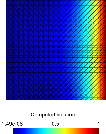
Differences
Linear and non-linear elasticity
This example uses a mesh that was generated with GiD. The object is meshed
with quadratic tetrahedrons. You can find the py-file of this example under
the name demo_tripod.py in the directory interface/tests/python/
of the GetFEM distribution.
 1import numpy as np
 2
 3import getfem as gf
 4
 5with_graphics=True
 6try:
 7    import getfem_tvtk
 8except:
 9    print("\n** Could NOT import getfem_tvtk -- graphical output disabled **\n")
10    import time
11    time.sleep(2)
12    with_graphics=False
13
14
15m=gf.Mesh('import','gid','../meshes/tripod.GiD.msh')
16print('done!')
17mfu=gf.MeshFem(m,3) # displacement
18mfp=gf.MeshFem(m,1) # pressure
19mfd=gf.MeshFem(m,1) # data
20mim=gf.MeshIm(m, gf.Integ('IM_TETRAHEDRON(5)'))
21degree = 2
22linear = False
23incompressible = False # ensure that degree > 1 when incompressible is on..
24
25mfu.set_fem(gf.Fem('FEM_PK(3,%d)' % (degree,)))
26mfd.set_fem(gf.Fem('FEM_PK(3,0)'))
27mfp.set_fem(gf.Fem('FEM_PK_DISCONTINUOUS(3,0)'))
28
29print('nbcvs=%d, nbpts=%d, qdim=%d, fem = %s, nbdof=%d' % \
30      (m.nbcvs(), m.nbpts(), mfu.qdim(), mfu.fem()[0].char(), mfu.nbdof()))
31
32P=m.pts()
33print('test', P[1,:])
34ctop=(abs(P[1,:] - 13) < 1e-6)
35cbot=(abs(P[1,:] + 10) < 1e-6)
36pidtop=np.compress(ctop, list(range(0, m.nbpts())))
37pidbot=np.compress(cbot, list(range(0, m.nbpts())))
38
39ftop=m.faces_from_pid(pidtop)
40fbot=m.faces_from_pid(pidbot)
41NEUMANN_BOUNDARY = 1
42DIRICHLET_BOUNDARY = 2
43
44m.set_region(NEUMANN_BOUNDARY,ftop)
45m.set_region(DIRICHLET_BOUNDARY,fbot)
46
47E=1e3
48Nu=0.3
49Lambda = E*Nu/((1+Nu)*(1-2*Nu))
50Mu =E/(2*(1+Nu))
51
52
53md = gf.Model('real')
54md.add_fem_variable('u', mfu)
55if linear:
56    md.add_initialized_data('cmu', Mu)
57    md.add_initialized_data('clambda', Lambda)
58    md.add_isotropic_linearized_elasticity_brick(mim, 'u', 'clambda', 'cmu')
59    if incompressible:
60        md.add_fem_variable('p', mfp)
61        md.add_linear_incompressibility_brick(mim, 'u', 'p')
62else:
63    md.add_initialized_data('params', [Lambda, Mu]);
64    if incompressible:
65        lawname = 'Incompressible Mooney Rivlin';
66        md.add_finite_strain_elasticity_brick(mim, lawname, 'u', 'params')
67        md.add_fem_variable('p', mfp);
68        md.add_finite_strain_incompressibility_brick(mim, 'u', 'p');
69    else:
70        lawname = 'SaintVenant Kirchhoff';
71        md.add_finite_strain_elasticity_brick(mim, lawname, 'u', 'params');
72
73
74md.add_initialized_data('VolumicData', [0,-1,0]);
75md.add_source_term_brick(mim, 'u', 'VolumicData');
76
77# Attach the tripod to the ground
78md.add_Dirichlet_condition_with_multipliers(mim, 'u', mfu, 2);
79
80print('running solve...')
81md.solve('noisy', 'max iter', 1);
82U = md.variable('u');
83print('solve done!')
84
85
86mfdu=gf.MeshFem(m,1)
87mfdu.set_fem(gf.Fem('FEM_PK_DISCONTINUOUS(3,1)'))
88if linear:
89  VM = md.compute_isotropic_linearized_Von_Mises_or_Tresca('u','clambda','cmu', mfdu);
90else:
91  VM = md.compute_finite_strain_elasticity_Von_Mises(lawname, 'u', 'params', mfdu);
92
93# post-processing
94sl=gf.Slice(('boundary',), mfu, degree)
95
96print('Von Mises range: ', VM.min(), VM.max())
97
98# export results to VTK
99sl.export_to_vtk('tripod.vtk', 'ascii', mfdu,  VM, 'Von Mises Stress', mfu, U, 'Displacement')
Here is the final figure, displaying the Von Mises stress and
displacements norms:
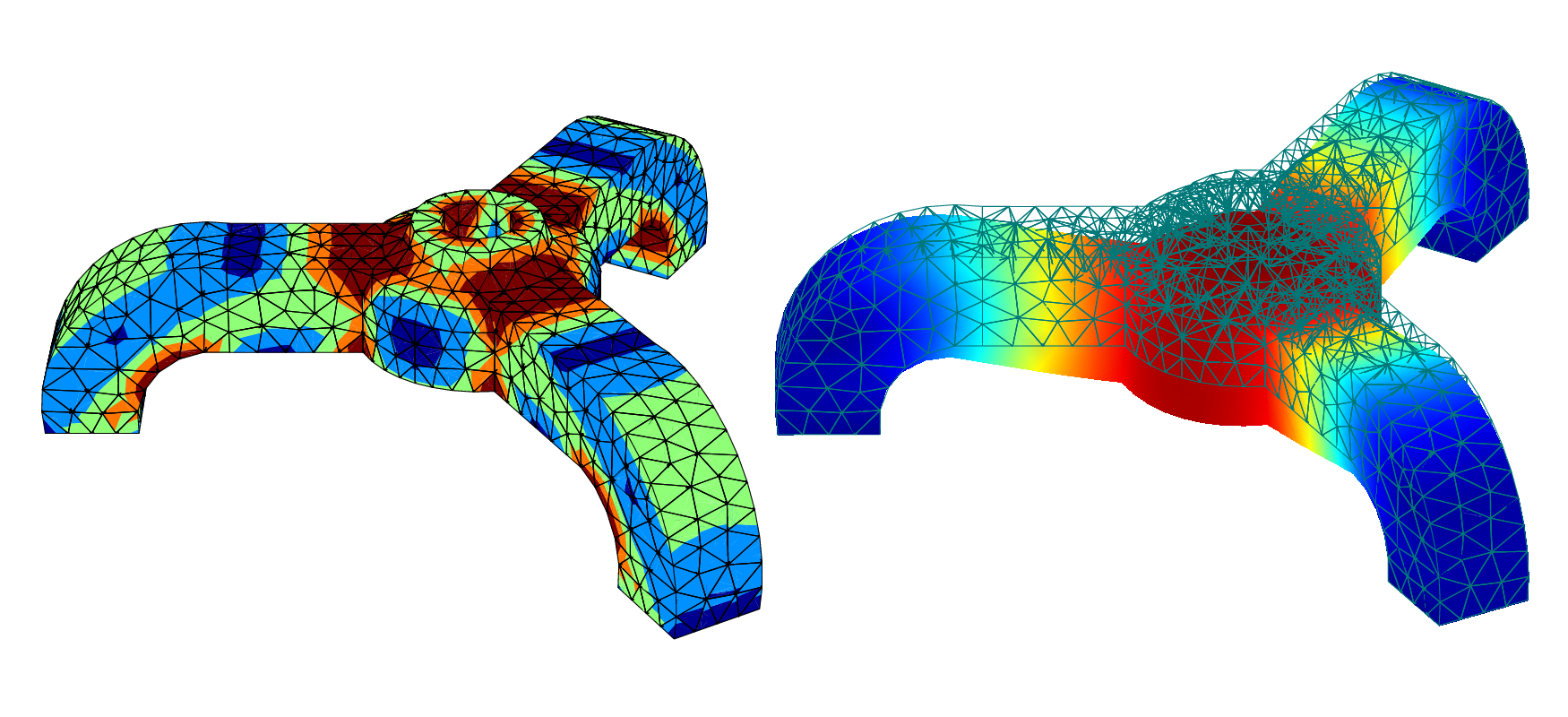
(a) Tripod Von Mises, (b) Tripod displacements norms.
Avoiding the model framework
The model bricks are very convenient, as they hide most of the details of the
assembly of the final linear systems. However it is also possible to stay at a
lower level, and handle the assembly of linear systems, and their resolution,
directly in Python. For example, the demonstration demo_tripod_alt.py is
very similar to the demo_tripod.py except that the assembly is explicit
mfu = gf.MeshFem(m,3) # displacement
mfe = gf.MeshFem(m,1) # for plot von-mises
mfu.set_fem(gf.Fem('FEM_PK(3,%d)' % (degree,)))
m.set_region(DIRICHLET_BOUNDARY,fbot)

# assembly
print "nbd: ",nbd

print "np.repeat([Mu], nbd).shape:",np.repeat([Mu], nbd).shape

# handle Dirichlet condition

print "U0.shape: ",U0.shape

Nt = gf.Spmat('copy',N)
Nt.transpose()
KK = Nt*K*N
FF = Nt*F # FF = Nt*(F-K*U0)

# solve ...
P = gf.Precond('ildlt',KK)
print "UU.shape:",UU.shape
print "U.shape:",U.shape

# post-processing
sl = gf.Slice(('boundary',), mfu, degree)

# compute the Von Mises Stress
DU = gf.compute_gradient(mfu,U,mfe)
VM = np.zeros((DU.shape[2],),'d')
Sigma = DU

for i in range(DU.shape[2]):
  d = np.array(DU[:,:,i])
  E = (d+d.T)*0.5
  Sigma[:,:,i]=E
  VM[i] = np.sum(E**2) - (1./3.)*np.sum(np.diagonal(E))**2
# can be viewed with mayavi -d ./tripod_ev.vtk -f WarpVector -m TensorGlyphs
#print 'mayavi -d ./tripod.vtk -f WarpVector -m BandedSurfaceMap'

# export to Gmsh
sl.export_to_pos('tripod.pos', mfe, VM,'Von Mises Stress', mfu, U, 'Displacement')
sl.export_to_pos('tripod_ev.pos', mfu, U, 'Displacement', SigmaSL, 'stress')
In getfem-interface, the assembly of vectors, and matrices is done via the gf.asm_*
functions. The Dirichlet condition \(h(x)u(x) = r(x)\) is handled in the
weak form \(\int (h(x)u(x)).v(x) = \int r(x).v(x)\quad\forall v\) (where
\(h(x)\) is a \(3\times 3\) matrix field – here it is constant and
equal to the identity). The reduced system KK UU = FF is then built via the
elimination of Dirichlet constraints from the original system. Note that it
might be more efficient (and simpler) to deal with Dirichlet condition via a
penalization technique.
Other examples
the
demo_refine.pyscript shows a simple 2D or 3D bar whose extremity is clamped. An adaptative refinement is used to obtain a better approximation in the area where the stress is singular (the transition between the clamped area and the neumann boundary).the
demo_nonlinear_elasticity.pyscript shows a 3D bar which is is bended and twisted. This is a quasi-static problem as the deformation is applied in many steps. At each step, a non-linear (large deformations) elasticity problem is solved.the
demo_stokes_3D_tank.pyscript shows a Stokes (viscous fluid) problem in a tank. Thedemo_stokes_3D_tank_draw.pyshows how to draw a nice plot of the solution, with mesh slices and stream lines. Note that thedemo_stokes_3D_tank_alt.pyis the old example, which uses the deprecatedgf_solvefunction.the
demo_bilaplacian.pyscript is just an adaption of the GetFEM exampletests/bilaplacian.cc. Solve the bilaplacian (or a Kirchhoff-Love plate model) on a square.the
demo_plasticity.pyscript is an adaptation of the GetFEM exampletests/plasticity.cc: a 2D or 3D bar is bended in many steps, and the plasticity of the material is taken into account (plastification occurs when the material’s Von Mises exceeds a given threshold).the
demo_wave2D.pyis a 2D scalar wave equation example (diffraction of a plane wave by a cylinder), with high order geometric transformations and high order FEMs.