Appendix B. Cubature method list
For more information on cubature formulas, the reader is referred to [EncyclopCubature] for instance. The integration methods are of two kinds. Exact integrations of polynomials and approximated integrations (cubature formulas) of any function. The exact integration can only be used if all the elements are polynomial and if the geometric transformation is linear.
A descriptor on an integration method is given by the function:
ppi = getfem::int_method_descriptor("name of method");
where "name of method" is a string to be chosen among the existing methods.
The program integration located in the tests directory lists and checks
the degree of each integration method.
Exact Integration methods
GetFEM furnishes a set of exact integration methods. This means that polynomials are integrated exactly. However, their use is (very) limited and not recommended. The use of exact integration methods is limited to the low-level generic assembly for polynomial \(\tau\)-equivalent elements with linear transformations and for linear terms. It is not possible to use them in the high-level generic assembly.
The list of available exact integration methods is the following
Exact Integration Methods
"IM_NONE()"Dummy integration method.
"IM_EXACT_SIMPLEX(n)"Description of the exact integration of polynomials on the simplex of reference of dimension
n.
"IM_PRODUCT(a, b)"Description of the exact integration on the convex which is the direct product of the convex in
aand inb.
"IM_EXACT_PARALLELEPIPED(n)"Description of the exact integration of polynomials on the parallelepiped of reference of dimension
n.
"IM_EXACT_PRISM(n)"Description of the exact integration of polynomials on the prism of reference of dimension
n
Even though a description of exact integration method exists on parallelepipeds or prisms, most of the time the geometric transformations on such elements are nonlinear and the exact integration cannot be used.
Newton cotes Integration methods
Newton cotes integration of order K on simplices, parallelepipeds
and prisms
are denoted by "IM_NC(N,K)", "IM_NC_PARALLELEPIPED(N,K)" and
"IM_NC_PRISM(N,K)" respectively.
Gauss Integration methods on dimension 1
Gauss-Legendre integration on the segment of order
K (with K/2+1 points)
are denoted by "IM_GAUSS1D(K)". Gauss-Lobatto-Legendre integration on the
segment of order K (with K/2+1 points) are denoted by
"IM_GAUSSLOBATTO1D(K)". It is only available for odd values of K. The
Gauss-Lobatto integration method can be used in conjunction with
"FEM_PK_GAUSSLOBATTO1D(K/2)" to perform mass-lumping.
Gauss Integration methods on dimension 2
Integration methods on dimension 2¶ graphic
coordinates (x, y)
weights
function to call / order
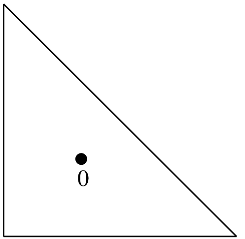
(1/3, 1/3)
1/2
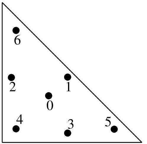
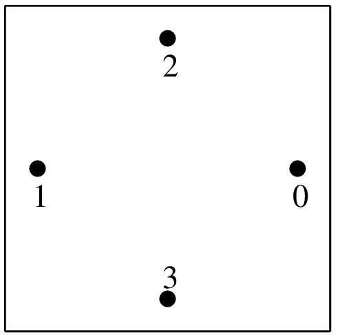
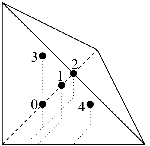
"IM_TRIANGLE(1)"1 point, order 1.
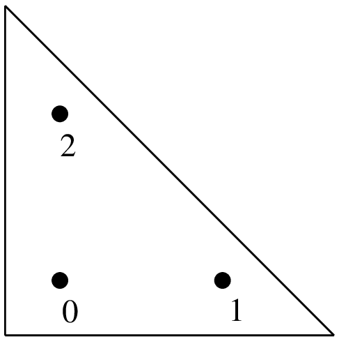
(1/6, 1/6)
(2/3, 1/6)
(1/6, 2/3)
1/6
1/6
1/6
"IM_TRIANGLE(2)"3 points, order 2.
Integration methods on dimension 2¶ graphic
coordinates (x, y)
weights
function to call / order
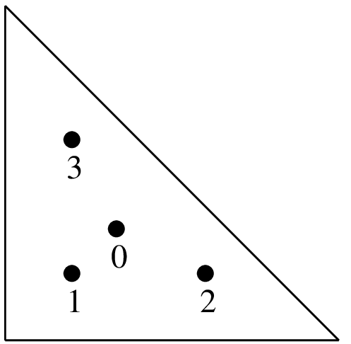
(1/3, 1/3)
(1/5, 1/5)
(3/5, 1/5)
(1/5, 3/5)
-27/96
25/96
25/96
25/96
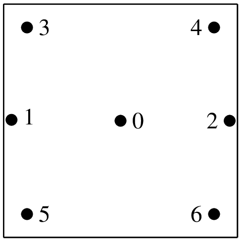
"IM_TRIANGLE(3)"4 points, order 3.
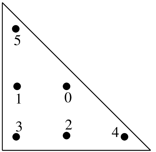
(a, a)
(1-2a, a)
(a, 1-2a)
(b, b)
(1-2b, b)
(b, 1-2b)
c
c
c
d
d
d
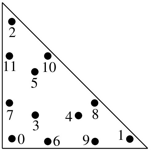
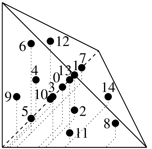
"IM_TRIANGLE(4)"6 points, order 4
\(a = 0.445948490915965\) \(b=0.091576213509771\) \(c=0.111690794839005\) \(d=0.054975871827661\)
(1/3, 1/3)
(a, a)
(1-2a, a)
(a, 1-2a)
(b, b)
(1-2b, b)
(b, 1-2b)
9/80
c
c
c
d
d
d
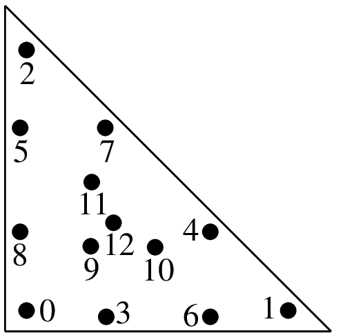
"IM_TRIANGLE(5)"7 points, order 5
\(a = \dfrac{6+\sqrt{15}}{21}\) \(b = 4/7 - a\) \(c = \dfrac{155+\sqrt{15}}{2400}\) \(d = 31/240 - c\)
(a, a)
(1-2a, a)
(a, 1-2a)
(b, b)
(1-2b, b)
(b, 1-2b)
(c, d)
(d, c)
(1-c-d, c)
(1-c-d, d)
(c, 1-c-d)
(d, 1-c-d)
e
e
e
f
f
f
g
g
g
g
g
g
"IM_TRIANGLE(6)"12 points, order 6
\(a = 0.063089104491502\) \(b = 0.249286745170910\) \(c = 0.310352451033785\) \(d = 0.053145049844816\) \(e = 0.025422453185103\) \(f = 0.058393137863189\) \(g = 0.041425537809187\)
Integration methods on dimension 2¶ graphic
coordinates (x, y)
weights
function to call / order
(a, a)
(b, a)
(a, b)
(c, e)
(d, c)
(e, d)
(d, e)
(c, d)
(e, c)
(f, f)
(g, f)
(f, g)
(1/3, 1/3)
h
h
h
i
i
i
i
i
i
j
j
j
k
"IM_TRIANGLE(7)"13 points, order 7
\(a = 0.0651301029022\) \(b = 0.8697397941956\) \(c = 0.3128654960049\) \(d = 0.6384441885698\) \(e = 0.0486903154253\) \(f = 0.2603459660790\) \(g = 0.4793080678419\) \(h = 0.0266736178044\) \(i = 0.0385568804451\) \(j = 0.0878076287166\) \(k = -0.0747850222338\)
"IM_TRIANGLE(8)"(see [EncyclopCubature])
"IM_TRIANGLE(9)"(see [EncyclopCubature])
"IM_TRIANGLE(10)"(see [EncyclopCubature])
"IM_TRIANGLE(13)"(see [EncyclopCubature])
(\(1/2+\sqrt{1/6}, 1/2\))
(\((1/2-\sqrt{1/24}, 1/2\pm\sqrt{1/8}\))
1/3
1/3
"IM_QUAD(2)"3 points, order 2
Integration methods on dimension 2¶ graphic
coordinates (x, y)
weights
function to call / order
(\(1/2\pm\sqrt{1/6}, 1/2\))
(\(1/2, 1/2\pm\sqrt{1/6}\))
1/4
1/4
"IM_QUAD(3)"4 points, order 3
(\(1/2, 1/2\))
(\(1/2 \pm \sqrt{7/30}, 1/2\))
(\(1/2\pm\sqrt{1/12}, 1/2\pm\sqrt{3/20}\))
2/7
5/63
5/36
"IM_QUAD(5)"7 points, order 5
"IM_QUAD(7)"12 points, order 7
"IM_QUAD(9)"20 points, order 9
"IM_QUAD(17)"70 points, order 17
There is also the "IM_GAUSS_PARALLELEPIPED(n,k)" which is a direct product of
1D gauss integrations.
Important note: do not forget that IM_QUAD(k) is exact for
polynomials up to degree \(k\), and that a \(Q_k\) polynomial has a degree
of \(2*k\). For example, IM_QUAD(7) cannot integrate exactly the product
of two \(Q_{2}\) polynomials. On the other hand,
IM_GAUSS_PARALLELEPIPED(2,4) can integrate exactly that product …
Gauss Integration methods on dimension 3
Integration methods on dimension 3¶ graphic
coordinates (x, y)
weights
function to call / order
(1/4, 1/4, 1/4)
1/6
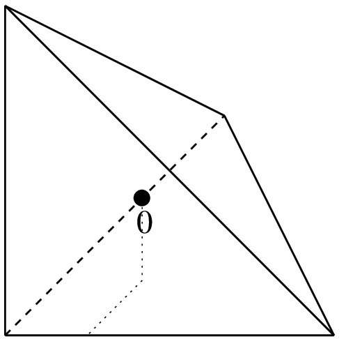
"IM_TETRAHEDRON(1)"1 point, order 1
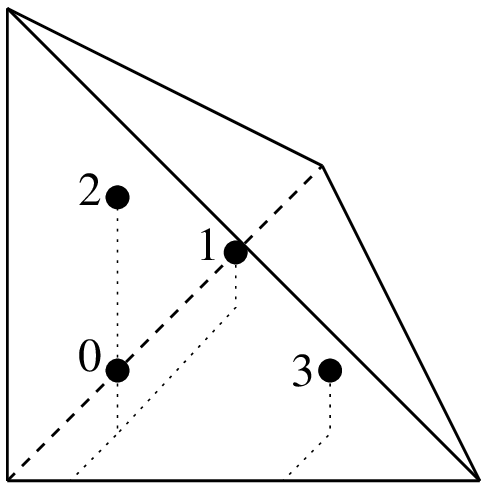
\((a, a, a)\)
\((a, b, a)\)
\((a, a, b)\)
\((b, a, a)\)
1/24
1/24
1/24
1/24
"IM_TETRAHEDRON(2)"4 points, order 2
\(a = \dfrac{5 - \sqrt{5}}{20}\)
\(b = \dfrac{5 + 3\sqrt{5}}{20}\)
Integration methods on dimension 3¶ graphic
coordinates (x, y)
weights
function to call / order
(1/4, 1/4, 1/4)
(1/6, 1/6, 1/6)
(1/6, 1/2, 1/6)
(1/6, 1/6, 1/2)
(1/2, 1/6, 1/6)
-2/15
3/40
3/40
3/40
3/40
"IM_TETRAHEDRON(3)"5 points, order 3
\((1/4, 1/4, 1/4)\)
\((a, a, a)\)
\((a, a, c)\)
\((a, c, a)\)
\((c, a, a)\)
\((b, b, b)\)
\((b, b, d)\)
\((b, d, b)\)
\((d, b, b)\)
\((e, e, f)\)
\((e, f, e)\)
\((f, e, e)\)
\((e, f, f)\)
\((f, e, f)\)
\((f, f, e)\)
8/405
\(h\)
\(h\)
\(h\)
\(h\)
\(i\)
\(i\)
\(i\)
\(i\)
5/567
5/567
5/567
5/567
5/567
5/567
"IM_TETRAHEDRON(5)"15 points, order 5
\(a = \dfrac{7 + \sqrt{15}}{34}\)
\(b = \dfrac{7 - \sqrt{15}}{34}\)
\(c = \dfrac{13 + 3\sqrt{15}}{34}\)
\(d = \dfrac{13 - 3\sqrt{15}}{34}\)
\(e = \dfrac{5 - \sqrt{15}}{20}\)
\(f = \dfrac{5 + \sqrt{15}}{20}\)
\(h = \dfrac{2665 - 14\sqrt{15}}{226800}\)
\(i = \dfrac{2665 + 14\sqrt{15}}{226800}\)
Others methods are:
name
element type
number of points
"IM_TETRAHEDRON(6)"tetrahedron
24
"IM_TETRAHEDRON(8)"tetrahedron
43
"IM_SIMPLEX4D(3)"4D simplex
6
"IM_HEXAHEDRON(5)"3D hexahedron
14
"IM_HEXAHEDRON(9)"3D hexahedron
58
"IM_HEXAHEDRON(11)"3D hexahedron
90
"IM_CUBE4D(5)"4D parallelepiped
24
"IM_CUBE4D(9)"4D parallelepiped
145
Direct product of integration methods
You can use "IM_PRODUCT(IM1, IM2)" to produce integration methods on
quadrilateral or prisms. It gives the direct product of two integration methods.
For instance "IM_GAUSS_PARALLELEPIPED(2,k)" is an alias for
"IM_PRODUCT(IM_GAUSS1D(2,k),IM_GAUSS1D(2,k))" and can be use instead of the
"IM_QUAD" integrations.
Specific integration methods
For pyramidal elements, "IM_PYRAMID(im)" provides an integration method corresponding to the transformation of an integration im from a hexahedron (for instance "IM_GAUSS_PARALLELEPIPED(3,5)") onto a pyramid. It is a singular integration method specically adapted to rational fraction shape functions of the pyramidal elements.
Composite integration methods
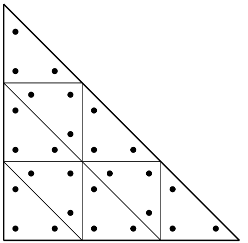
Composite method "IM_STRUCTURED_COMPOSITE(IM_TRIANGLE(2), 3)"
Use "IM_STRUCTURED_COMPOSITE(IM1, S)" to copy IM1 on an element with S
subdivisions. The resulting integration method has the same order but with more
points. It could be more stable to use a composite method rather than to improve
the order of the method. Those methods have to be used also with composite
elements. Most of the time for composite element, it is preferable to choose the
basic method IM1 with no points on the boundary (because the gradient could be
not defined on the boundary of sub-elements).
For the HCT element, it is advised to use the "IM_HCT_COMPOSITE(im)" composite
integration (which split the original triangle into 3 sub-triangles).
For pyramidal elements, "IM_PYRAMID_COMPOSITE(im)" provides an integration method ase on the decomposition of the pyramid into two tetrahedrons (im should be an integration method on a tetrahedron). Note that the integraton method "IM_PYRAMID(im)" where im is an integration method on an hexahedron, should be prefered.